Wave3D
The Wave3D is a software of the time-domain boundary element meted (TDBEM) for the 3D wave equation.
- Wave3D is fast
- The method is accelerated by a variant of the fast multipole method (FMM), which is similar to the planewave time-domain (PWTD) algorithm but more algebraic rather than analytic because it exploits the interpolation-based FMM. The computational complexity of the fast TDBEM is O(Ns^(1+f)*Nt), while that of the conventional TDBEM is O(Ns^2*Nt), where the number f is 1/3 or 1/2 (according to the spatial distribution of the boundary elements) and Ns and Nt denote the spatial and temporal DOFs, respectively. The details are described in the paper in JCP.
- Wave3D is memory-efficient
- The FMM can result in a less amount of memory than the conventional TDBEM. This feature is useful when you solve large-scale problems.
- Wave3D is parallelizable
- The Wave3D can be parallelized with OpenMP on a shared-memory machine. Thus, you can fully utilize all the computing cores on your PC. The parallelization on a distributed computing system has not been considered yet.
- Wave3D is general-purpose
- Wave3d can handle arbitrary-shaped surface(s) in a computational domain. In the case of external problems, where the computational domain spreads infinitely Here, we do NOT have to consider any absorbing boundary condition (ABC) on the boundary of the domain. You can give Dirichlet and/or Neumann boundary condition on such one or more closed surfaces. In addition, you can program the incident field that you want, e.g., planewave, point source.
- Wave3D is getting stable
- This is a result of the recent progress on the time stabilization of the TDBEM; see the paper in arXiv. The stabilization is indispensable when one solves external Dirichlet problems, while the external Neumann problem, which has been mainly considered so far, is not serious for the stability.
Example 1: FMM vs Conventional method
The following table shows a numerical result to solve an external Neumann problem, where the scatter is discretized with 13,240 boundary elements and the number of time steps is 480. Here, "Conv." stands for the conventional TDBEM and the number following "FMM" denotes the precision parameter. First of all, the FMM is >10x faster than the conventional method, where both methods are parallelized with 20 cores on dual Xeon E5-2687W. In addition, you can see that the precision parameter can control the trade-off between speed (as well as memory) and accuracy.
| Method | Time [s] | Speedup | Relative error | Memory [GB] |
| Conv. | 20159 | 1.0 | na | 203 |
| FMM(6) | 1084 | 18.6 | 2.0e-2 | 17 |
| FMM(8) | 1105 | 18.2 | 1.2e-2 | 18 |
| FMM(10) | 1305 | 15.4 | 6.6e-3 | 21 |
| FMM(12) | 1897 | 10.6 | 5.2e-3 | 26 |

Example 2: Room acousitics
As another example, the animation of Figure 18 in the JCP paper is found here. You can see the sound generated in the RHS room at t=0 propagates to the LHS room and the outside through the windows and door. In the animation, the outer surfaces are removed to see the inside of the house.

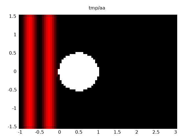
Example 3: Scattering by a sphere
It is possible to compute the sound pressure at any point. This computation is also accelerated by the FMM. This example demonstrates such a calcuation. Specifically, we considered a scattering problem due to a acoustically-soft sphere when a continuous pulse is impinged to it. The sound pressure on a cross section (width 4 and height 3) including the center of the sphere is available as the animation. The number of boundary elements and interior points are 5120 and 4428, respectively, while the number of time steps is 400. The computation time was about 292 second with the above-mentioned 20 cores.
 time step. This picture was created by Gnuplot in a stupid way. So the jaggy boundary profile is not a true one, which is spanned with 5120 triangles. It should be noted that the computational domain is INFINITE and the sound pressure can be computed at any point --- the present FMBEM inherits all the advantages of the BEM!")
HOME